Week 7 workshop

Week 7 Workshop

Izzy Tector

# should haves
library(tidyverse)
library(here)
library(lterdatasampler)
# would be nice to have
# performance allows us to check the performance of our models
library(performance)
library(broom)
# flextable allows us to make tables
library(flextable)
# ggeffects allows us to get predictions for models
library(ggeffects)
library(car)
library(naniar)

Linear Models

how does stem length predict stem dry mass

maples_data <- hbr_maples %>% 
  # & does the same as a comma would do in this case
  filter(year == 2003 & watershed == "Reference")

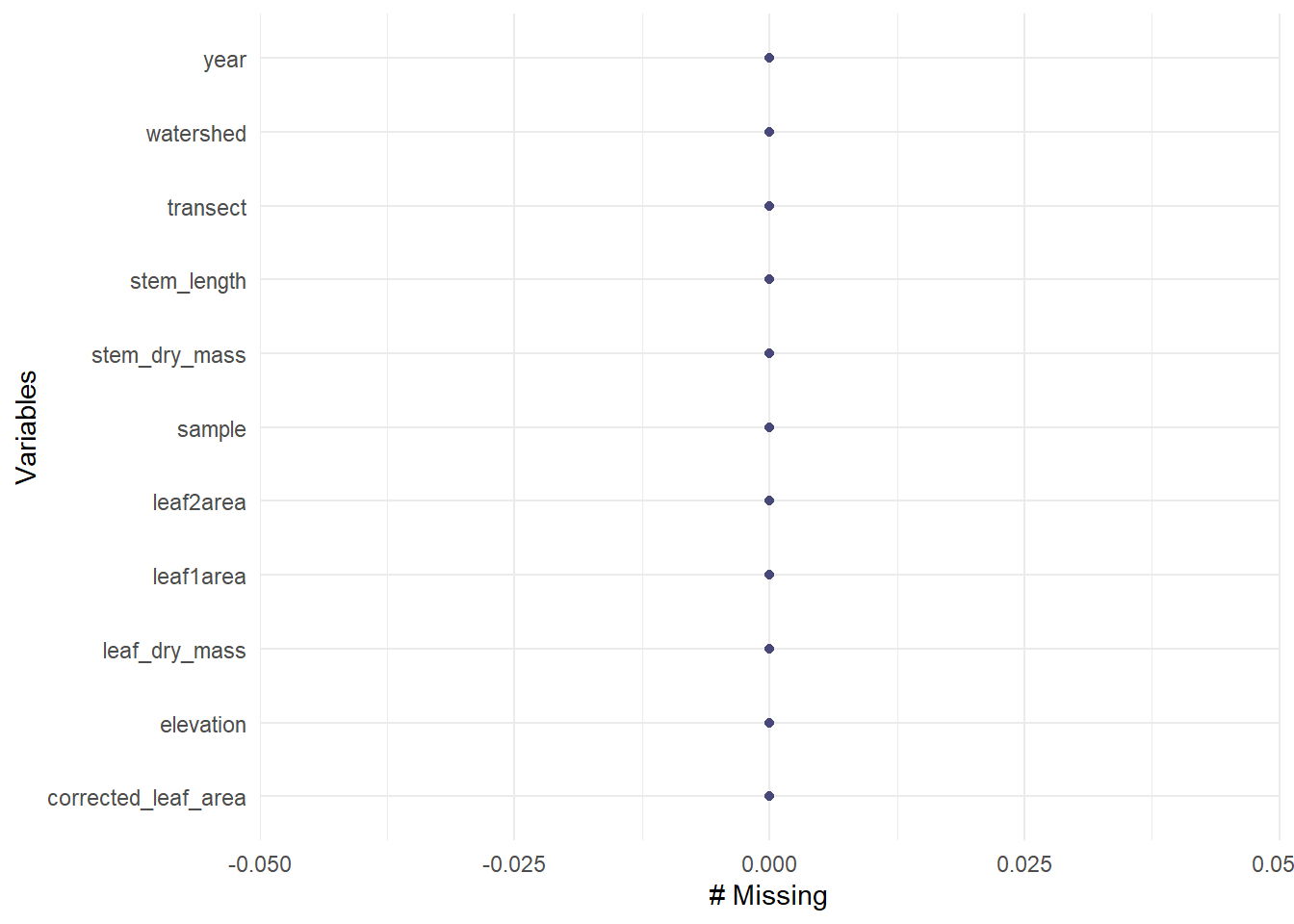
visualizing missing data

gg_miss_var(maples_data)

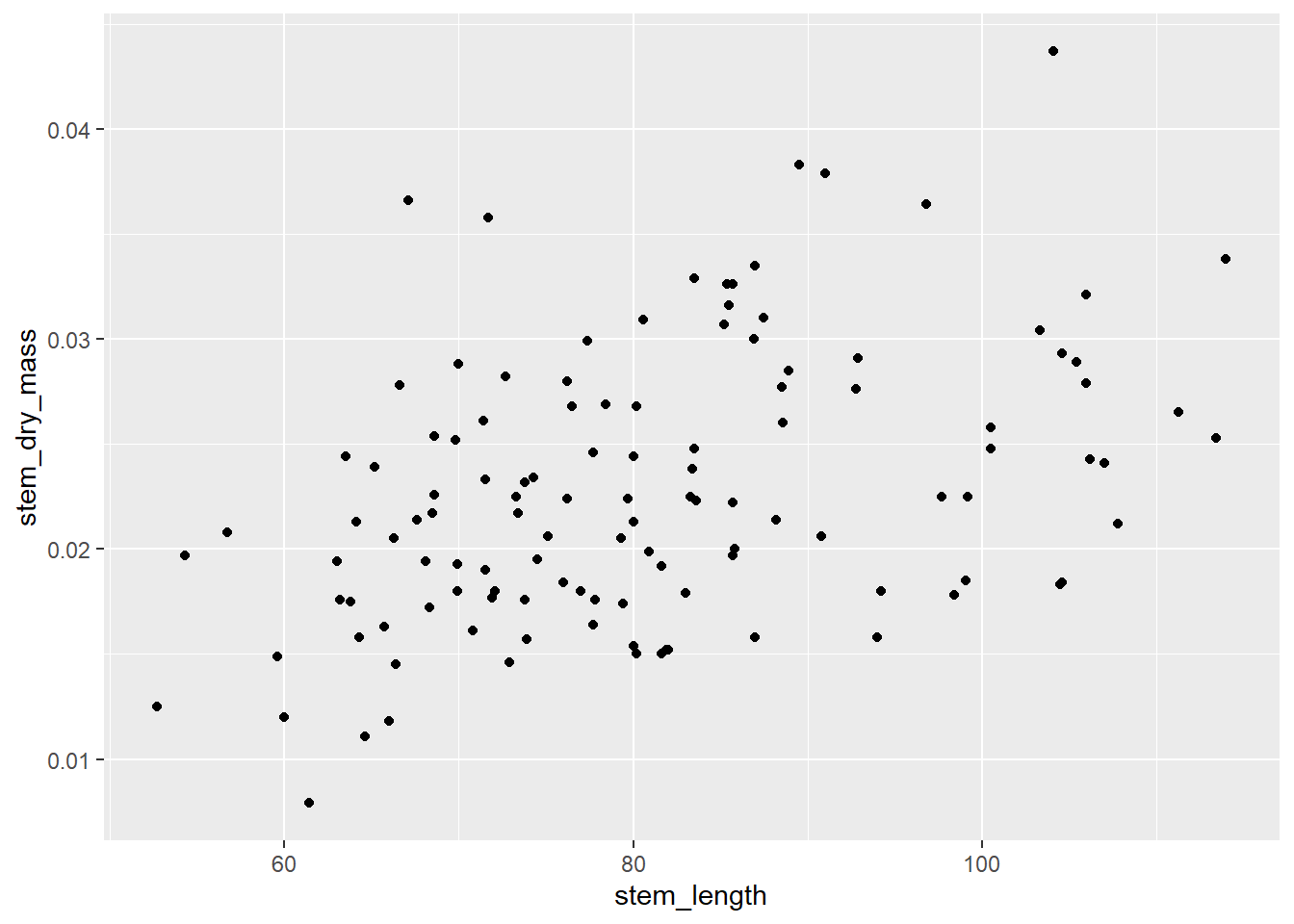
creating an exploratory data visualization

ggplot(data = maples_data, aes(x = stem_length, y = stem_dry_mass)) + 
  geom_point()

lets try a model

# we are going to be resuign this model a binch of times so it would be smart to make it an object
# lm makes a linear model
# for lm you put the y axis and what it is predicting after ~
maples_model <-  lm(stem_dry_mass ~ stem_length, data = maples_data)

maples_model

Call:
lm(formula = stem_dry_mass ~ stem_length, data = maples_data)

Coefficients:
(Intercept)  stem_length  
  0.0070033    0.0001958  

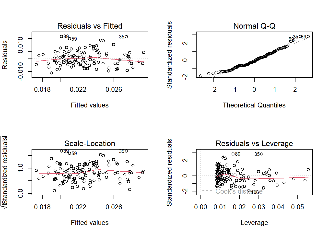
check our assumptions

1. linear relationship between variables: yes! (used the exploratory data visualization to check that)
2. independence of errors: yes! (making that assumption based on how the data were collected)
3. homoskedasticity: yes! (making that decision from residuals vs fitted plot/scale-location plots)
4. normally distributed errors: yes! (looking at QQ plot of residuals)

# par allows us to set up a grid, preset in R, sets graphical parameters
par(mfrow = c(2, 2))
plot(maples_model)

turn off the 2 by 2 grid

dev.off()

null device 
          1